---
title: "How much of Denver can walk to frequent transit?"
subtitle: "A SQL and R analysis of RTD's weekday service, from the morning peak to late night"
author: "Austin Foster"
date: today
---
```{r}
#| label: setup
#| include: false
library(dplyr)
library(tidyr)
library(ggplot2)
library(readr)
source("R/config.R")
out <- "output"
m <- read_csv(file.path(out, "headline_metrics.csv"), show_col_types = FALSE) |> arrange(period_order)
routes <- read_csv(file.path(out, "route_headways.csv"), show_col_types = FALSE)
stops <- read_csv(file.path(out, "stop_frequency.csv"), show_col_types = FALSE)
access_file <- file.path(out, "access_by_period.csv")
has_access <- file.exists(access_file)
if (has_access) acc <- read_csv(access_file, show_col_types = FALSE)
walkshed_file <- file.path(out, "frequent_walksheds.geojson")
has_walksheds <- file.exists(walkshed_file)
feed_date <- if (file.exists("data/raw/download_date.txt")) readLines("data/raw/download_date.txt") else "unknown"
pct <- function(x) paste0(format(x, nsmall = 1), "%")
fmt_min <- function(x) ifelse(x == round(x), sprintf("%.0f", x), sprintf("%.1f", x))
num <- function(x) format(x, big.mark = ",")
# one value for one period, e.g. by_period(m, "Late Night", routes_frequent)
by_period <- function(df, p, col, key = "period") dplyr::pull(df[df[[key]] == p, ], {{ col }})
period_factor <- function(x) factor(x, levels = PERIODS)
service_day <- format(m$service_date[1], "%A, %B %d, %Y")
```
## Executive summary
<!-- EDIT: rewrite these sentences in your own voice once the numbers are in. -->
On a typical weekday (`r service_day`), RTD ran `r m$routes_all_day[1]` routes.
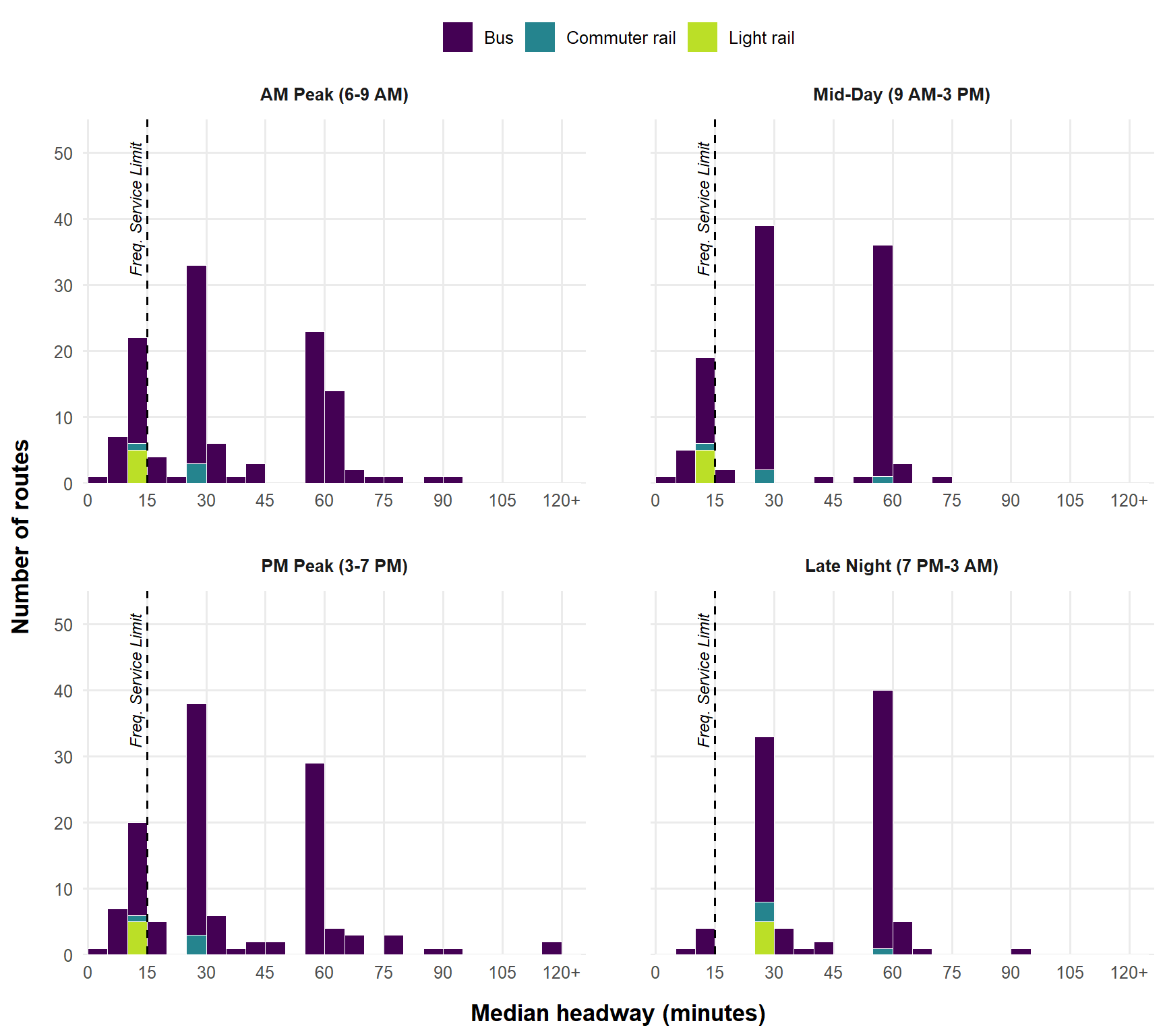
Counting a route as **frequent** when its median gap between trips is 15 minutes or less in both directions, **`r by_period(m, "AM Peak", routes_frequent)`** routes were frequent in the AM peak (6–9 AM), **`r by_period(m, "Mid-Day", routes_frequent)`** at mid-day, and **`r by_period(m, "PM Peak", routes_frequent)`** in the PM peak, but only **`r by_period(m, "Late Night", routes_frequent)`** between 7 PM and 3 AM.
Of the `r num(m$stops_served_all_day[1])` stops served that day, `r pct(by_period(m, "AM Peak", pct_stops_frequent))` had frequent service in the AM peak and `r pct(by_period(m, "Late Night", pct_stops_frequent))` late at night.
```{r}
#| results: asis
#| echo: false
if (has_access) {
a <- function(p, col) by_period(acc, p, {{ col }}, key = "walkshed")
cat(sprintf(
"About **%s of residents** in the seven RTD counties, and **%s of households without a car**, live within a quarter-mile walk of a frequent stop in the AM peak. After 7 PM that falls to **%s** and **%s**.",
pct(a("AM Peak", pct_pop_near)), pct(a("AM Peak", pct_zero_car_near)),
pct(a("Late Night", pct_pop_near)), pct(a("Late Night", pct_zero_car_near))))
}
```
## Why this matters
Frequency is what turns a bus line into something people can use without planning around it. When a bus comes every 15 minutes or better, riders can walk to the stop and go, a missed trip costs minutes rather than an hour, and transfers between routes become practical. Service that runs less often forces people to build their day around a timetable, which is a burden most drivers never face. That burden falls hardest on people without a car, who rely on transit for work, school, groceries, and appointments, and whose trips don't all happen at rush hour. Measuring where frequent service exists, and when it disappears, shows which neighborhoods have transit they can count on all day and which have it only at the peaks.
## Data
| Source | What it provides | Version |
|---|---|---|
| [RTD GTFS feed](https://www.rtd-denver.com/open-records/open-spatial-information/gtfs) | Every scheduled trip, stop, and departure time | Downloaded `r feed_date` |
| [ACS 5-year estimates](https://www.census.gov/programs-surveys/acs) (tables B01003, B25044) | Population and households without a vehicle, by block group | 2019–2023 |
| [OpenStreetMap](https://www.openstreetmap.org/copyright) via [Geofabrik](https://download.geofabrik.de/north-america/us/colorado.html) | Streets, sidewalks, and paths for walking distances | Downloaded with the GTFS run |
## Method
1. **Load** the GTFS text files into DuckDB, a SQL database that runs inside R.
2. **Pick a typical weekday.** GTFS covers months of service, so the SQL expands the calendar into individual dates, applies holiday exceptions, and chooses the Wednesday with the most scheduled trips.
3. **Split the day into four periods:** AM Peak (6–9 AM), Mid-Day (9 AM–3 PM), PM Peak (3–7 PM), and Late Night (7 PM–3 AM). GTFS writes after-midnight times as 24:00 or later, so Late Night ends at 27:00. Trips between 3 and 6 AM fall outside the four periods.
4. **Measure route headways** (`sql/03_route_headways.sql`). For each route and direction, a `LAG()` window function finds the time between successive trips at the stop the route serves most often. Only gaps between two trips that **both leave inside the same period** count. A gap that runs across a period boundary, or from the last trip of the night to 3 AM, is left out. A route is **frequent** in a period if its **median** headway is 15 minutes or less in every direction, with at least 4 trips each way (an hour's worth at 15 minutes). The median is the typical scheduled gap: half the gaps are shorter, half are longer, so one odd gap at a service change doesn't decide the result.
5. **Flag frequent stops** (`sql/04_stop_frequency.sql`). The same calculation runs at every stop. A stop is frequent in a period if a single route-direction serving it has a median headway of 15 minutes or less there, with at least 4 departures. Several infrequent routes stacked together don't count, because riders can't combine them into one wait.
6. **Build walksheds on the street network** (`R/04_osm_network.R`, `R/05_walksheds.R`). OpenStreetMap streets, sidewalks, and paths become a routable network. One shortest-path search per period finds everywhere within a quarter-mile **walk** of a frequent stop, so rail lines, highways, and dead ends limit access the way they do on foot.
7. **Estimate who lives nearby** (`R/06_census_access.R`). ACS block groups are counted in proportion to how much of their area falls inside each period's walkshed.
## Results
### Service by time of day
For each route running in a period, the SQL takes the median gap between its trips in its less frequent direction. @tbl-periods reports the median of those values across the whole system, so every route counts once however often it runs. Half of RTD's routes come at least this often.
```{r}
#| label: tbl-periods
#| tbl-cap: "Median scheduled headway across all RTD routes, by time of day"
m |>
  transmute(
    Period = PERIOD_LABELS[period],
    `Median headway (min)` = fmt_min(system_median_headway_min)
  ) |>
  knitr::kable(align = "lr")
```
### How often do routes run?
```{r}
#| label: fig-headways
#| fig-cap: "Median headway by route and time of day (weaker direction). Routes at or left of the dashed line run every 15 minutes or better. Routes with a single trip in a period have no headway and are not shown."
#| fig-height: 8
#| fig-width: 9
hw <- routes |>
  filter(!is.na(median_headway_min)) |>
  mutate(
    median_headway_min = pmin(median_headway_min, 120),
    period = factor(PERIOD_LABELS[period], levels = PERIOD_LABELS)
  )

# The threshold label ends at y = 51.5 in every panel.
threshold_lab <- tibble(period = factor(PERIOD_LABELS, levels = PERIOD_LABELS),
                        y = 51.5)

ggplot(hw, aes(median_headway_min, fill = mode)) +
  geom_histogram(binwidth = 5, boundary = 0, color = "white", linewidth = 0.2) +
  geom_vline(xintercept = 15, linetype = "dashed") +
  geom_text(data = threshold_lab, aes(x = 15, y = y), inherit.aes = FALSE,
            label = "Freq. Service Limit", angle = 90,
            hjust = 1, vjust = -0.5, size = 3.2, fontface = "italic") +
  # scales = "free_x" draws an x-axis under every panel; the fixed limits
  # keep all four panels on the same 0-120+ scale so they stay comparable
  facet_wrap(~ period, ncol = 2, scales = "free_x") +
  scale_x_continuous(limits = c(0, 125), breaks = seq(0, 120, 15),
                     labels = c(seq(0, 105, 15), "120+"), expand = expansion(mult = 0.01)) +
  # headroom above the tallest bars so the vertical label fits
  scale_y_continuous(limits = c(0, 55), breaks = seq(0, 50, 10), expand = expansion(mult = 0)) +
  scale_fill_viridis_d(option = "viridis", end = 0.9) +
  labs(x = "Median headway (minutes)", y = "Number of routes", fill = NULL) +
  theme_minimal(base_size = 12) +
  theme(legend.position = "top",
        strip.text = element_text(face = "bold", margin = margin(b = 10)),
        axis.title = element_text(face = "bold", size = 13),
        axis.title.x = element_text(margin = margin(t = 12)),
        axis.title.y = element_text(margin = margin(r = 12)),
        panel.spacing.x = unit(2.5, "lines"),   # room between the two columns of panels
        panel.spacing.y = unit(1.8, "lines"),
        panel.grid.minor = element_blank())
```
### The frequent routes
Each cell shows the route's median headway in that period, in its less frequent direction, using only gaps between trips that leave inside the period. **Bold** marks periods where the route is frequent; a dash means no service (or a single trip) in that period. The shortest and longest gaps for each route and period are in [Additional Data](additional-data.qmd).
```{r}
#| label: tbl-frequent
#| tbl-cap: "Routes that are frequent in at least one period: median headway in minutes"
fmt <- function(x) ifelse(x == round(x), sprintf("%.0f", x), sprintf("%.1f", x))
frequent_ids <- routes |> filter(is_frequent) |> distinct(route_id)
routes |>
  semi_join(frequent_ids, by = "route_id") |>
  filter(!is.na(median_headway_min)) |>
  mutate(cell = fmt(median_headway_min),
         # asterisk: the median isn't a standard clock-face headway
         cell = ifelse(median_headway_min %in% STANDARD_HEADWAYS, cell, paste0(cell, "\\*")),
         cell = ifelse(is_frequent, paste0("**", cell, "**"), cell),
         period = period_factor(period)) |>
  group_by(route_id) |>
  mutate(n_frequent = sum(is_frequent), best = min(median_headway_min)) |>
  ungroup() |>
  select(route_id, Route = route_short_name, Name = route_long_name, Mode = mode,
         n_frequent, best, period, cell) |>
  pivot_wider(names_from = period, values_from = cell, values_fill = "–") |>
  arrange(desc(n_frequent), best) |>
  select(Route, Name, Mode, any_of(PERIODS)) |>
  knitr::kable(align = "lllrrrr")
```
\* The median isn't a standard clock-face headway (3, 4, 5, 6, 7.5, 10, 12, 15, 20, 30, 45, 60, or 90 minutes), so riders won't see the same minutes past the hour all period. Usually the route mixes two headways in the period, such as alternating 7 and 8 minutes or switching between 15 and 30. See [Additional Data](additional-data.qmd) for each route's shortest and longest gap.
### Where is frequent service?
```{r}
#| label: fig-map
#| fig-cap: "Frequent stops and their quarter-mile walksheds by time of day. Use the layer button (top right) to switch periods or turn on aerial imagery. Click a stop for its headways."
library(leaflet)
library(sf)
period_cols <- setNames(viridisLite::viridis(4, end = 0.9), PERIODS)

stop_popup <- stops |>
  mutate(txt = case_when(
    routes_in_period == 0         ~ "no service",
    is.na(best_median_headway_min) ~ "fewer than 4 trips",
    TRUE                           ~ paste0(best_median_headway_min, " min"))) |>
  group_by(stop_id) |>
  summarise(popup = paste0("<b>", htmltools::htmlEscape(first(stop_name)), "</b><br>",
                           "<i>Best route, median headway</i><br>",
                           paste0(period, ": ", txt, collapse = "<br>")), .groups = "drop")
all_stops <- stops |> distinct(stop_id, stop_lat, stop_lon) |> left_join(stop_popup, by = "stop_id")

map <- leaflet() |>
  # Keyless tile layers. (CARTO basemaps started requiring an API key in 2026,
  # which is why the old map showed "API key required".)
  addProviderTiles(providers$Esri.WorldGrayCanvas, group = "Light") |>
  addProviderTiles(providers$Esri.WorldImagery,    group = "Aerial imagery") |>
  addProviderTiles(providers$OpenStreetMap,        group = "Streets") |>
  addCircleMarkers(data = all_stops, lng = ~stop_lon, lat = ~stop_lat,
                   radius = 1.5, color = "#8C8C8C", stroke = FALSE, fillOpacity = 0.5,
                   popup = ~popup, group = "All stops")

if (has_walksheds) {
  sheds <- st_read(walkshed_file, quiet = TRUE) |>
    filter(walkshed %in% PERIODS) |>
    st_transform(PROJECTED_CRS) |>
    st_simplify(dTolerance = 15, preserveTopology = TRUE) |>   # lighter web page
    st_transform(4326)
}

for (p in PERIODS) {
  grp <- PERIOD_LABELS[[p]]
  shed_p <- if (has_walksheds) filter(sheds, walkshed == p, !st_is_empty(geometry)) else NULL
  if (!is.null(shed_p) && nrow(shed_p) > 0) {
    map <- map |>
      addPolygons(data = shed_p, group = grp,
                  color = period_cols[[p]], weight = 1, fillOpacity = 0.25,
                  options = pathOptions(interactive = FALSE))   # clicks pass through to stops
  }
  map <- map |>
    addCircleMarkers(data = filter(stops, period == p, is_frequent) |>
                       left_join(stop_popup, by = "stop_id"),
                     lng = ~stop_lon, lat = ~stop_lat, radius = 3.5,
                     color = period_cols[[p]], stroke = FALSE, fillOpacity = 0.9,
                     popup = ~popup, group = grp)
}

map |>
  addLegend(colors = c(unname(period_cols), "#8C8C8C"),
            labels = c(unname(PERIOD_LABELS), "Other stops"),
            title = "Frequent service", opacity = 1) |>
  addLayersControl(baseGroups = c("Light", "Aerial imagery", "Streets"),
                   overlayGroups = c(unname(PERIOD_LABELS), "All stops"),
                   options = layersControlOptions(collapsed = TRUE)) |>
  hideGroup(unname(PERIOD_LABELS[-1]))     # start with AM Peak only
```
### Who lives near frequent service?
A worker on a 9-to-5 schedule only needs the peaks. Someone who heads to work in the afternoon and comes home at midnight needs frequent service in both directions of that trip, so their access is capped by the Late Night row.
```{r}
#| label: tbl-access
#| tbl-cap: "Residents and households without a car within a quarter-mile walk of a frequent stop, by time of day"
#| echo: false
if (has_access) {
acc |>
filter(walkshed %in% c(PERIODS, "Every period")) |>
mutate(walkshed = factor(walkshed, levels = c(PERIODS, "Every period"))) |>
arrange(walkshed) |>
transmute(
Period = ifelse(walkshed %in% PERIODS, PERIOD_LABELS[as.character(walkshed)],
"All four periods"),
Residents = num(pop_near_frequent),
`Share of residents` = pct(pct_pop_near),
`Households without a car` = num(zero_car_hh_near),
`Share of car-free households` = pct(pct_zero_car_near)
) |>
knitr::kable(align = "lrrrr")
} else {
cat("Run R/04_osm_network.R through R/06_census_access.R to add this section.")
}
```
```{r}
#| results: asis
#| echo: false
if (has_access && "AM Peak (straight-line)" %in% acc$walkshed) {
a <- function(p, col) by_period(acc, p, {{ col }}, key = "walkshed")
cat(sprintf(
"For comparison, the straight-line quarter-mile circles used in an earlier version of this analysis would have counted **%s** of residents in the AM peak instead of **%s**. Measuring along the street network matters most where freeways, rail lines, and cul-de-sacs sit between people and the stop.",
pct(a("AM Peak (straight-line)", pct_pop_near)), pct(a("AM Peak", pct_pop_near))))
}
```
## Limitations
- **Walk network.** OpenStreetMap is very complete in metro Denver, but it often draws a street with sidewalks as one centerline, so the analysis assumes every street is walkable on both sides and ignores how hard it is to cross a wide arterial.
- **Areal weighting** assumes people are spread evenly across each block group.
- **One day, scheduled service.** Results describe scheduled service on one Wednesday, not weekends or actual on-time performance.
- **The median describes the typical gap, not the worst one.** A route that runs every 15 minutes for most of a period and every 30 for the rest counts as frequent, though riders arriving during the 30-minute stretch wait longer. The min–max range in the frequent-routes table shows when that happens.
- **Gaps are measured only inside each period.** A route that runs every 10 minutes from 6 to 7 AM and then stops still counts as frequent for the AM Peak, because the wait after its last trip isn't counted. The 4-trip minimum keeps a pair of closely spaced trips (such as a school tripper) from qualifying on its own.
- **Route headways are measured at one stop** (the one each route serves most often). The stop-level results use actual departure times at every stop, so they also capture short-turn trips that never reach that stop.
- **Late Night crosses midnight.** Trips that leave between midnight and 3 AM on the service day are treated as the end of the previous night's service.
## Reproduce this
```bash
git clone https://github.com/austinthomas7/rtd-frequent-network
```
Then run `R/00_setup.R` once, `run_all.R`, and `quarto render`. All code is on [GitHub](https://github.com/austinthomas7/rtd-frequent-network).